Planning a trajectory means defining a sequence of poses in 3D space. These defined poses are interpolated in order to result in a smooth and continuous curve. Most beautiful are cubic Bézier curves.

Bézier curves are polynoms of 3^rd grade using a start and an end point and two support points defining the curvature at the start and end point. The trajectory is defined by the start and the end point, the support point is not on the trajectory but used to make it smooth only. The computation is based on a parameter t=0..1 defining the ratio of how much the current position has already made of the full curve. Let’s assume, we have the four points P₀..P₃, of which P₁ and P₂ are support points the curve does not touch:

    

This computation is done for x, y, and z coordinates. Although being beautiful, Bézier curves have a tendency to “bounce”, if the support points P₁ and P₂ differ too much in terms of the distance to the trajectory points P₀ and P₃. So, it is necessary to normalize support points by a small trick:

The picture illustrates a trajectory defined by A, B, C, and D. We want to model the piece between B and C with a cubic Bézier curve.

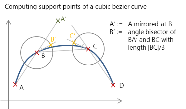
The support point B’ is computed by taking point A, mirroring it at B (A’), and moving along the angle bisector of A’ B C by a 1/3 of the length of BC, C’ is computed in an analogous manner.

This approach is rather arbitrary, but results in a smooth and non-oscillating curve. On the left, we see a linear trajectory, on the right the same curve as bezier curve. All this is implemented in BezierCurve.cpp.

Now the curve looks fine, but simply following that curve is not enough to make a smooth movement. We need a speed profile that avoids jerky movements. This is done by speed profiles. The classical approach is to use trapezoidal speed profiles like this:

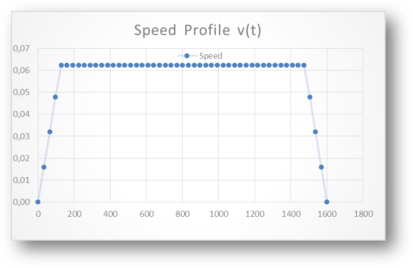
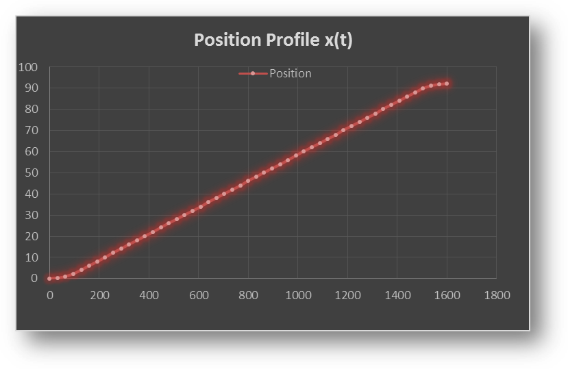
This trapezoid speed profile results in a constant (maximum) acceleration, then continuing with no acceleration, and a constant deceleration until zero speed is reached. To get the position on a curve, speed is integrated over time

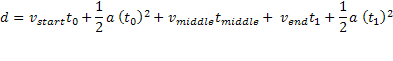
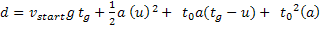
Despite of the corners in the speed profile, the position profile looks smooth. Still, how is a profile like that computed? Having a constant acceleration a, start speed v_start, an end speed v_end, the distance d (length of the Bezier curve) and the desired duration of the complete profile t_g, we need to compute the time t₀ and t₁ which is the duration of the starting acceleration and final deceleration. The full distance is given by

    

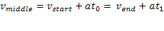
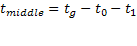
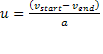
The duration and speed of the plateau is given by

         

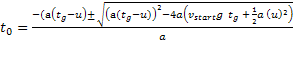
Rearranging these equations to get t₀ ends up in

    

with

    

Finally, with the equation above we get

    

With the equation above on computing d we get t_g.

This holds true for a trapezoid profile only, since to model a full trajectory that consist of single movements we also need profiles that represent a ramp or stairways, depending on the constrains in terms of duration, distance, and start/end speed. This ended up in quite a lot of code treating all the different cases.

On the right, the effect of a speed profile is illustrated compared to the same trajectory without speed profile. The effect is not spectacular, but can be detected when watching the top left and bottom left corner: On the left, the movement is continous. On the right, the movement stops slowly and accelerates when it continues.Speed profiles are implemented in SpeedProfile.cpp.

All this is done while planning a trajectory, so it is done upfront. At runtime, the trajectory is fully compiled and contains bezier curves and speed profiles already. The according UI where trajectories are planned looks like this (source code is WalterPlanner)

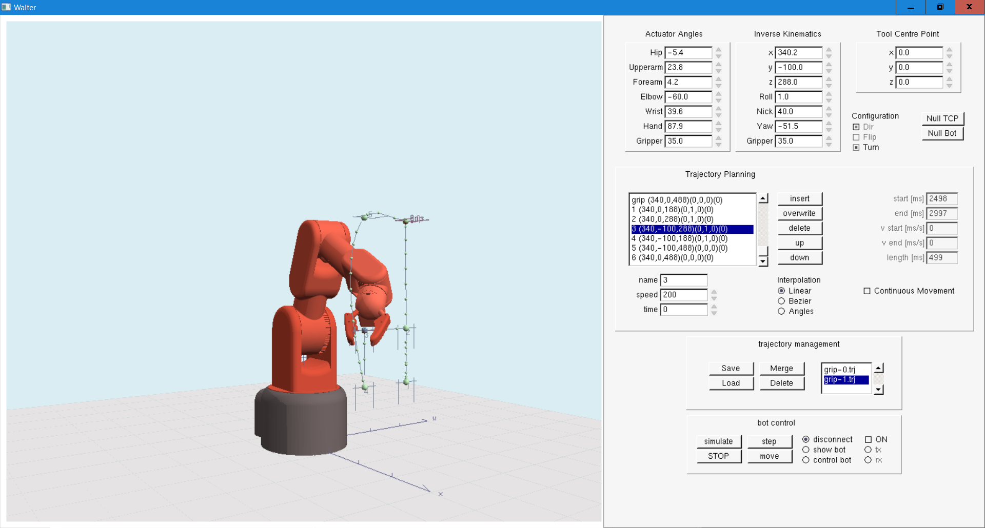
This UI provides forward and inverse kinematics (explained in Kinematics), allows to define a trajectory by defining support points (indicated by big green balls). After having assigned some parameters like speed or duration the trajectory is compiled, i.e. the bezier curves and speed profiles are computed (indicated by small green balls). This trajectory can be send to Walter to be executed by its Cortex.

Now we have a nice trajectory with a smooth speed profile, but do not yet know how to compute the angles of the joints.

This is explained in Kinematics and will be tough to read, take your time.